measure_adj: A software package for making measurements and computing adjoint sources for seismic tomography
Note
This is a remake version of measure_adj manual, which credited by Carl Tape, Qinya Liu
Introduction
Note
This is a preliminary user manual with many modifications to come.
The open-source software package measure_adj is designed for making measurements for seismic tomography. Several misfit functions are available, such as a simple waveform difference, a simple cross-correlation traveltime difference, or a frequency dependent multitaper traveltime difference. For each misfit function, the code also provides adjoint sources, which are needed for tomographic inversions using adjoint methods [Tromp et al., 2005, Liu and Tromp, 2006, Tape et al., 2007]. This code was used to make measurements and adjoint sources for the (large-scale) tomographic inversion of Tape et al. [2009] for the southern California crust.
MEAS–ADJ is designed to complement FLEXWIN [Maggi et al., 2009], which is designed to pick time windows for measurement. In particular, FLEXWIN has the option of providing a MEASUREMENT.WINDOWS file that can be directly read into measure_adj. However, FLEXWIN is not necessary to run measure_adj.
There are two additional sets of notes on multitaper measurements and adjoint sources, multitaper_notes.pdf and multitaper_vala.pdf. Some sections of multitaper_notes.pdf were published as “Multitaper measurements for adjoint tomography” in Appendix C [Tape, 2009].
Please email Carl Tape: carltape@fas.harvard.edu with suggestions or corrections.
Getting started
System requirements
In order to install and run, measure_adj program requires:
UNIX operating system (Linux, Solaris, MacOS …)
GNU make
a fortran compiler (gfortran, ifort, etc…)
other packages : SAC (Seismic Analysis Code, available from IRIS); GMT (Generic Mapping Tools) for the plotting scripts
MEAS–ADJ requires the following libraries external to the package in order to compile and run: libsacio.a and libsac.a. Both libraries are distributed by IRIS as part of the SAC package (version 101.2 and above). The IRIS download site (as of 21-Oct-2009) is here. (To check your version, type sac.)
Obtaining the code
Note
The code is available as a gzipped tarball from CIG (Computational Infrastructure for Geodynamics, \url{http://www.geodynamics.org}). The tarball is unpacked by typing tar xvzf flexwin.tgz.
(Use SVN for now.)
The package contains the MEAS–ADJ code and documentation, as well as a set of test data, examples of user files for different scenarios, and a set of utility scripts that may be useful for running measure_adj on large datasets.
Compilation
If your compiler of choice is gfortran, then you should be able to use the Makefile with only minor modifications (notably you may need to change the search path for the libsacio.a library). If you prefer another compiler, you should modify the OPT and FC lines in the makefiles accordingly. We tested the code using gfortran version 4.3.3. (To check your version, type gfortran --version.)
Steps to compile the MEAS–ADJ package:
make clean
make
You should end up with the measure_adj executable.
Running the test case
After compiling, execute the following two commands:
measure_adj
csh -f run_mt_measure_adj.csh
If all goes well, you should generate the figure
PLOTS/9818433_T006_T030_MPM_CI_m16_mtm_win_adj.pdf
A set of auxillary programs/files are required for the successful run of post-processing and plotting scripts, including
Southern California faults xy files in
PLOTS/plot_win_adj.pl:$dir0 = "/opt/seismo/datalib/SC/"; $fault_file = "$dir0/jennings.xy";
Dr. Lupei Zhu’s
saclstprogramDr. Lupei Zhu’s
pssac2plotting program (pssacmay work as well).
Running MEAS–ADJ
Two input files are read in when mt_measure_adj is executed.
Input file 1: MEASUREMENT.WINDOWS
3
DATA/9818433.CI.MPM.BHR.sac.d.T006_T030
SYN/MPM.CI.BHR.semd.sac.m16.T006_T030
           3
   11.2770    58.4770
   58.4770    81.3770
   81.3770   101.6770
DATA/9818433.CI.MPM.BHT.sac.d.T006_T030
SYN/MPM.CI.BHT.semd.sac.m16.T006_T030
           1
   49.3270    95.3270
DATA/9818433.CI.MPM.BHZ.sac.d.T006_T030
SYN/MPM.CI.BHZ.semd.sac.m16.T006_T030
           1
   60.9770    99.3770
The first line contains the number of pairs of records to be read in. Each pair of files is followed by the number of windows within which measurements will be made, followed by the time intervals for each window.
Note that data and synthetics require to have exactly the same t0, dt, npts for the code to run through. Therefore
no interpolation of dt is really necessary at any point.
Input file 2: MEASUREMENT.PAR
  -0.585 0.0110   18200  # tstart, DT, npts: time vector for simulations
                      7  # imeas (1-8; see manual)
                     BH  # channel of synthetics: BH or LH
      30.000      6.000  # TLONG and TSHORT: band-pass periods for records
                .false.  # RUN_BANDPASS: use band-pass on records
                 .true.  # DISPLAY_DETAILS
                 .true.  # OUTPUT_MEASUREMENT_FILES
                 .true.  # COMPUTE_ADJOINT_SOURCE
     -4.5000     4.5000  # TSHIFT_MIN; TSHIFT_MAX
     -1.5000     1.5000  # DLNA_MIN; DLNA_MAX
                  0.690  # CC_MIN
                      1  # ERROR_TYPE -- 0 none; 1 CC, MT-CC; 2 MT-jack-knife (all for MTM!)
                  1.000  # DT_SIGMA_MIN: water level of traveltime uncertainty
                  0.500  # DLNA_SIGMA_MIN: water level of dlnA uncertainty
                      1  # ITAPER:1 multi-taper; 2 cosine; 3 boxcar taper type for freq-dep. meas.
            0.020  2.50  # WTR, NPI (ntaper = 2*NPI)
                  2.000  # DT_FAC (following 4 pars are for MTM --> CC check)
                  2.500  # ERR_FAC
                  3.500  # DT_MAX_SCALE
                  1.500  # NCYCLE_IN_WINDOW
The names below correspond to the variable names in mt_measure_adj (see subroutine read_par_file in mt_sub.f90).
Time vector:
tt(start time),dtt(time step),nn(number of points). These values are particularly important if adjoint sources are requested. Based on the convention in SPECFEM3D, for example, it is best to select the start time to be \(t_0 = -1.5 \tau_{\rm h}\), where \(\tau_{\rm h}\) is the half duration of the CMT source. The time step and the number of time steps should exactly match the time file of the SPECFEM3D synthetics.Option for measurement:
imeas0= 1–8 (see Measurement options).Channel:
chanis BH or LH (based on options for SEM synthetics).Bandpass range:
TLONG(long-period),TSHORTshort-periodRUN_BANDPASS: whether to bandpass the seismograms.OUTPUT_MEASUREMENT_FILES: whether to output measurement files for each window.Limits on cross-correlation measurement:
TSHIFT_MIN;TSHIFT_MAX. These can optionally be read in from thePAR_FILEused in the FLEXWIN algorithm.Limits on amplitude measurement:
DLNA_MIN;DLNA_MAX. These can optionally be read in from thePAR_FILEused in the FLEXWIN algorithm.Limits on the cross-correlation measurement:
CC_MIN. This can optionally be read in from thePAR_FILEused in the FLEXWIN algorithm.ERROR_TYPE= 0–2: Type of estimated errors associated with \blue{multi-taper} measurement (and adjoint source). No error (0), cross-correlation error estimate (1), multitaper jack-knife error estimate (2). The cross-correlation error estimate is presented in Appendix A [Tape et al., 2010]. Forimeas=5,6 (cc),sigma_dt/dlnA_ccis automatically used. ForERROR_TYPE = 0, allsigma_tauandsigma_dlnAare set to be 1 for multitaper adjoint sources.DT_SIGMA_MIN: water-level minimum cross-correlation traveltime difference uncertainty estimate.DLNA_SIGMA_MIN: water-level minimum amplitude difference uncertainty estimate.Multitaper parameter,
ITAPER: Type of taper to use in constructing the transfer function between synthetics and data. Taper options are multitaper (1), cosine taper (2), and boxcar taper (3). For the single-taper options (2–3) the transfer function is not used, as the adjoint sources are constructed directly from the synthetic seismograms. For the multitaper option, the number of tapers is fixed to be twiceNPI(see multitaper_vala.pdf).Multitaper parameters,
WTR,NPI(see multitaper_vala.pdf).
Note
WTR is also used to determine i_right corresponding to the maximum frequency of valid frequency-dependent measurements. It requires
that the power at this frequency is above 10 times the WTR*max_syn_power.
Multitaper parameter,
DT_FAC(see Multitaper parameters).Multitaper parameter,
ERR_FAC(see Multitaper parameters).Multitaper parameter,
DT_MAX_SCALE(see Multitaper parameters).Multitaper parameter,
NCYCLE_IN_WINDOW, (see Multitaper parameters).
Multitaper parameters
The selection of the multitaper parameters DT_FAC, ERR_FAC, DT_MAX_SCALE, and NCYCLE_IN_WINDOW are not easy for each particular dataset. These parameters determine whether a multitaper measurement is reasonable enough to retain (otherwise revert to a cross-correlation measurement). The key subroutine is mt_measure_select.f90.
MTMs are rejected (user_trace = .false.) based on:
number of cycles in the window
number of frequency points given within
[fstart,fend]. Even whenRUN_BANDPASSis turned off, theTLONGandTSHORTare still converted tofstart,fend. They are best set to the values used inFLEXWINtshift_cc <= dt: too small a time shiftabs(dtau_w(j)) > Tvec(j)/DT_FAC: \(\tau\) at a specific frequency is too higherr_dt(j) > Tvec(j)/ERR_FAC: error for a specific frequency is too highabs(dtau_w(j)) > DT_MAX_SCALE*abs(tshift))\(\tau\) at specific frequency deviates too much for globaltshift_cc
Note
The cross-correlation measurements are then run through cc_measure_select() to determine if they are usable or not (tshift, dlnA = 0).
Two example sets of parameters are given
! ********* adjust following for global traces ************************
  ! ratio of current period with respect to dt and err_dt measurements
  double precision, parameter :: DT_FAC = 1.0
  double precision, parameter :: ERR_FAC = 8.0
  ! max time shift allowed at all freq should be DT_MAX_SCALE * Tshift_xc
  double precision, parameter :: DT_MAX_SCALE = 5.0
  ! few cycles for surfaces waves
  double precision, parameter :: NCYCLE_IN_WINDOW = 2.0 ! window length > 2.*50
!***********************************************************************

! ********* adjust following for socal 3-30s traces ********************
  ! ratio of current period with respect to dt and err_dt measurements
  double precision, parameter :: DT_FAC = 2.0
  double precision, parameter :: ERR_FAC = 2.5
  ! max time shift allowed at all freq should be DT_MAX_SCALE * Tshift_xc
  double precision, parameter :: DT_MAX_SCALE = 3.5
  ! use 3 cycles for surfaces waves
  double precision, parameter :: NCYCLE_IN_WINDOW = 1.5
!***********************************************************************
Output files
There are two output files related to measurements in the local run directory:
window_chi, a comprehensive output file of misfit values, with one line per window.
! KEY: write misfit function values to file (for each window)
! Here are some columns of values in window_chi (add 8 for the actual column number)
!  1: MT-TT chi (imeas=7),    2: MT-dlnA chi (imeas=8)
!  3: XC-TT chi (imeas=5),    4: XC-dlnA chi (imeas=6)
!  5: MT-TT meas (freq-average),   6: MT-dlnA meas,   7: XC-TT meas,   8: XC-dlnA meas
!  9: MT-TT error, 10: MT-dlnA error, 11: XC-TT error, 12: XC-dlnA error
! WINDOW     : 13: data power, 14: syn power, 15: (data-syn) power, 16: window duration
! FULL RECORD: 17: data power, 18: syn power, 19: (data-syn) power, 20: record duration
! WINDOW     : 21: tr_chi,       22: am_chi
! Example of a reduced file: awk '{print $2,$3,$4,$5,$6,$29}' window_chi > window_tr_chi

write(13,'(a14,a8,a3,a5,i4,i4,2e14.6,20e14.6,2e14.6,2f14.6)') &
   file_prefix0,sta,net,chan_syn,j,imeas,&
   tstart,tend,window_chi(:),tr_chi,am_chi,T_pmax_dat,T_pmax_syn

! misfit function value
if(is_mtm==1) window_chi(1) = 0.5 * 2.0 * df * sum( (dtau_w(1:i_right))**2 * wp_taper(1:i_right) ) ! tr_chi
if(is_mtm==1) window_chi(2) = 0.5 * 2.0 * df * sum( (dlnA_w(1:i_right))**2 * wq_taper(1:i_right) ) ! amp_chi
window_chi(3) = 0.5 * (tshift/sigma_dt_cc)**2 ! tr_chi
window_chi(4) = 0.5 * (dlnA/sigma_dlnA_cc)**2 ! amp_chi
! cc/averaged-mt tshift/dlnA measurement
if(is_mtm==1) window_chi(5)  = sum( dtau_w(1:i_right) * w_taper(1:i_right) ) / sum(w_taper(1:i_right) )
if(is_mtm==1) window_chi(6)  = sum( dlnA_w(1:i_right) * w_taper(1:i_right) ) / sum(w_taper(1:i_right) )
window_chi(7) = tshift
window_chi(8) = dlnA
! estimated measurement uncertainties
if(is_mtm==1) window_chi(9) = sigma_dt
if(is_mtm==1) window_chi(10) = sigma_dlnA
window_chi(11) = sigma_dt_cc
window_chi(12) = sigma_dlnA_cc
! for normalization, divide by duration of window
window_chi(13) = 0.5 * sum(dat_dtw(:)**2)
window_chi(14) = 0.5 * sum(syn_dtw(:)**2)
window_chi(15) = 0.5 * sum((dat_dtw-syn_dtw)**2) ! tr/amp_chi for imeas=1/2
window_chi(16) = nlen*dt
window_chi(17) = 0.5 * sum( data**2 ) ! power of entire trace
window_chi(18) = 0.5 * sum( syn**2 )
window_chi(19) = 0.5 * sum( (data-syn)**2 )
window_chi(20) = npts*dt
window_index, an abbreviated output file with the indexing for each window. The columns are
write(12,'(a3,a8,a5,a5,3i5,2f12.3)') net,sta,chan_syn,chan_dat,nwin,ipair,j,tstart,tend
where nwin is the overall window counter, ipair is the seismogram (pair) counter, and j is the local window counter. For example, for the test case run:
CI MPM     BHR  BHR      1    1    1      11.277      58.477
CI MPM     BHR  BHR      2    1    2      58.477      81.377
CI MPM     BHR  BHR      3    1    3      81.377     101.677
CI MPM     BHT  BHT      4    2    1      49.327      95.327
CI MPM     BHZ  BHZ      5    3    1      60.977      99.377
With COMPUTE_ADJOINT_SOURCE = .true.,
adjoint source files (e.g.,
MPM.CI.BHZ.iker07.adj) will appear inOUTPUT_FILES/. These are ascii files with the time colume defined bytstart,DT,nptsin the parameter file. (ifDO_RAY_DENSITY_SOURCE = .true., adjoint file names areMPM.CI.BHZ.iker7.density.adj).window_chi_sumin local directory, the sum of misfit values (CC or MTM) of all windows, with weights taken into account ifDO_WEIGHTING = .true.. This scalar value literally corresponds to all the adjoint sources produced inOUTPUT_FILES/. If input includes all windows for a particular event, this scalar value is the event misfit. More comprehensive sum of misfit can be found in the script/ADJOINT_TOMO/iterate_adj/matlab/compute_misfit.m
With OUTPUT_MEASUREMENT_FILES = .true. in MEASUREMENT.PAR, you should find numerous output files in OUTPUT_FILES/.
Other files include (prefix=MPM.CI.BHZ.01.mtm, prefix0=MPM.CI.BHZ)
prefix.recon_syn_cc.sac             # syn_dtw_cc
prefix.recon_syn_cc_dt.sac          # syn_dtw_cc_dt
prefix.dt/dlnA_average/cc           # dtau/dlnA_meas, dtaul/dlnA_sigma ('average' means 'mtm')
prefix.ph/abs/dlnA/ph_cor/dt        # transfer fun.:  phi/abs/log(abs)/phi(corr)/dtau(idf_new:idf_new:i_right)
                                    #                 tshift/dlnA from cc are added to dtau/dlnA_wt
prefix.recon_syn.sac                # recon. syn with both dtau(om) and dlnA(om) applied for all imeas >=3 cases.
prefix.recon_syn_dt.sac             # reconstructed syn with only dtau(om) applied
prefix.err_ph/abs/dt/dlnA[_full]    # err_phi/abs/dt/dlnA_mtm(idf_new:idf_new:i_right)
prefix.freq_limits                  # fstart/fend (input),df, fstart/fend(adjusted for given window)
prefix0.recon.sac                   # recon. syn after applying CC or MTM for the entire data trace
If DISPLAY_MORE_DETAILS = .true. in the parameter file, following files will be written for every window pair
prefix.obs (original data/syn)
prefix.syn
prefix.dat.sac (time windowed data/syn)
prefix.syn.sac
prefix.obs.power % abs(dat_dtwo(1:i_right)), i.e., dat_dtw_cc
prefix.syn.power % abs(syn_dtwo(1:i_right)), i.e., syn_dtw
Scripts
The three scripts in the run directory are
write_par_file.pl. Write the fileMEASUREMENT.PARfrom a given set of parameters. This is called within the run scripts inscripts_tomo.prepare_adj_src.pl. This script reads in a set of adjoint sources made from Z-R-T records and outputs a set of adjoint sources in Z-E-N that can be used in SPECFEM3D.
prepare_adj_src.pl -m CMT -z BH -s STATION -o OUTDIR -i [rotation] all_adj_ZRT_files
prepare_adj_src.pl -m CMTSOLUTION_9818433 -s PLOTS/STATIONS_TOMO -o ADJOINT_SOURCES \
                   OUTPUT_FILES/*adj
It loops over all the stations with adjoint sources present in OUTPUT_FILES, and write an associate STATION_ADJOINT to local dir. It also rotates adjoint sources to E-N-Z, and deposits them into ADJOINT_SOURCES dir.
The key is that it will create an all-zeros record if no measurement is made on a particular component (say, Z), but IS made on another component (say, R or T). It uses the following fortran program:
rotate_adj_src baz(radian!) zfile tfile rfile efile nfile
The perl script also outputs STATIONS_ADJOINT file for all the stations with adjoint sources.
combine_adj_src.pl. This script combines two sets of adjoint sources (for example, two different bandpassed versions), and outputs the new adjoint sources, along with a newSTATIONS_ADJOINTfile to be used.
Usage: combine_adj_src.pl DIR_1 DIR_2 DIR_NEW imeas1 imeas2 chan
Adjoint sources from dir1 and dir2 with the same station/net/component names are added up; station files from dir1/STATIONS_ADJOINT anddir2/STATIONS_ADJOINT are combined into dir_new/STATIONS_ADJOINT.
Scripts in the PLOT/ directory:
The primary plotting script is
PLOTS/plot_win_adj.pl.
plot_win_adj_all.pl -m CMTFILE -a STATION_FILE -n chan -b iboth -l tmin/tmax \
    -k imeas/iadj -d data_dir -s syn_dir -c recon_dir -w winfile -i smodel -j Tmin/Tmax
plot_win_adj_all.pl -l -10/200 -m ../CMTSOLUTION_9818433 -n BH -b 0 -k 7/1 \
    -a STATIONS_ADJOINT -d DATA -s SYN -c RECON -w MEASUREMENT.WINDOWS -i m16 -j 6/30
which uses another script
plot_win_adj.pl -m $cmtfile -n $sta/$net/$chan -b $iboth -l $tcuts -k $opt_k \
   -a $station_list -d $data_dir -s $syn_dir -c $recon_dir -w $winfile -i $smodel -j $Ts
plot_win_adj.pl -m ../CMTSOLUTION_9818433 -n MPM/CI/BH -b 0 -l -10/200 -k 7/1 \
   -a STATIONS_ADJOINT -d DATA -s SYN -c RECON -w MEASUREMENT.WINDOWS -i m16 -j 6/30
gives plots of detailed information on data, syn, reconstructed syn and corresponding adjoint sources, as well as
source/station distributions on a map (Figure Left: Data (black), synthetics (red), and measurement windows.
Right: Adjoint sources for a multitaper traveltime difference (imeas = 7). for MTM, imeas=7)
Some tweaking is probably necessary before successful application to a different dataset, including: setting evid in CMT file (correspond to data name evid.net.sta), setting corresponding kstnam,knetwk,kcmpnm for both data and synthetics, setting o header properly, and all synthetics need to be present (data/recon-syn not needed).
plot the statistics of window files (check file structure before use)
plot_win_stats_all.pl Tmin/Tmax model iplot [plot histogram or not]
plot_win_stats.pl Tmin/Tmax eid name meas_file sta_file eid_text cmtall_psmeca
organize
plot_win_adj_all.ploutput by station or event (???)
make_pdf_by_event.pl
make_pdf_by_station.pl
For large datasets, we have included an additional set of scripts in the directory
scripts_tomo. Each user will have to make some modifications to these scripts.For plotting output files for individual measurements, we have included a set of scripts in
scripts_meas. These scripts have not been extensively tested.
Measurement options
There are several choices of measurements (or definitions of misfit functions), and each choice leads to a different adjoint source, as illustrated in Tromp et al. [2005]. The user must specify a value of imeas in MEASUREMENT.PAR with the following options:
imeas = 1, normalized waveform difference. Adjoint source is constructed from the data only, with the form \(-d(t)/\|d(t)\|^2\).\[\phi = \frac{1}{2}\frac{\int [d(t)-s(t)]^2\,dt }{\int d^2(t)\,dt} \quad \text{at}\quad s(t)=0\]\[f^\dagger(t) = -\frac{d(t)}{\|d(t)\|^2}\]If
NO_WAVEFORM_DIFFERENCE = .true., this becomes (why???)\[f^\dagger(t) = d(t)\]imeas = 2, waveform difference, \(s(t) - d(t)\).\[\phi = \frac{1}{2}\int [d(t)-s(t)]^2\,dt\]\[f^\dagger(t) = s(t)-d(t)\]imeas = 3, cross-correlation traveltime for a (banana-doughtnut) sensitivity kernel. The measurement between data and synthetics is not used in constructing the adjoint source.\[\phi = T_{syn}\]\[\delta \phi = \delta{T_{syn}} = - \frac{\int w(t) \dot{s}(t) \delta s(t)\,dt}{\int w(t) \dot{s}^2(t)\,dt} \quad\quad\quad\text{TTL (43)}\]\[f^\dagger(t) = -\frac{w(t)\dot{s}(t)}{\int w(t) \dot{s}^2(t)\,dt}\]where \(w(t)\) is the time window over which the measurement is made.
imeas = 4, amplitude difference for a (banana-doughtnut) sensitivity kernel. The measurement between data and synthetics is not used in constructing the adjoint source.\[\phi = \ln A_{syn}\]\[\delta \phi = \delta ln A_{syn} = \frac{\int w(t)s(t)\delta s(t)\,dt}{\int w(t) s^2(t)\,dt} \quad\quad\quad\text{TTL (64)}\]\[f^\dagger(t) = \frac{w(t) s(t)}{\int w(t) s^2(t)\,dt}\]imeas = 5, cross-correlation traveltime difference for an event kernel.\[\phi = \frac{1}{2}\sum_{rp}\left[ \frac{T_{obs}-T_{syn}}{\sigma_{\Delta T}} \right]^2 \]\[\delta \phi = - \sum_{rp} \frac{T_{obs}-T_{syn}}{\sigma^2_{\Delta T}}\, \delta{T_{syn}} = \sum_{rp} \frac{ \Delta T_{syn}}{\sigma^2_{\Delta T}} \frac{\int w(t) \dot{s}(t) \delta s(t)\,dt}{\int w(t) \dot{s}^2(t)\,dt}\]\[f^\dagger(t) = \sum_{rp} \frac{w(t)\dot{s}(t)}{\int w(t) \dot{s}^2(t)\,dt} \frac{ \Delta T_{syn}}{\sigma^2_{\Delta T}}\]where the traveltime delay of observed data w.r.t. synthetics \(\Delta T_{syn}= T_{obs}-T_{syn}\) is used in constructing the adjoint source. The summation is performed over receivers (\(r\)) and phases (\(p\)).
Note the cross-correlation related measurements, including
tshift, dlnA, cc_maxgiven bycompute_syn_cc()correspond to\[cc_i = \frac{\sum_j s_j d_{j+i}}{\sum_j s_j s_j},\quad \Delta T = i_{max}*dt, \quad \Delta \ln A = \frac{1}{2} \ln \left[\frac{\int d^2(t) dt}{\int s^2(t) dt}\right],\]and average error estimates are given by
\[\sigma_{\Delta T} = \sqrt{\frac{\int[d(t)-s_c(t)]^2\,dt}{\int \dot{s}^2_c(t)\,dt}},\quad \sigma_{\Delta lnA} = \sqrt{\frac{\int[d(t)-s_c(t)]^2\,dt}{\int s^2_{ct}(t)\,dt}}\]
where \(s_c(t)\) is the reconstructed synthetics after applying \(\Delta T\) and \(\Delta \ln A\) corrections.
imeas = 6, amplitude difference for an event kernel. As\[d(t) \sim \exp(\Delta \ln A)\, s(t) \sim (1+\Delta \ln A_{syn})\, s(t)\]the misfit of amplitude anomaly may be defined by
\[\phi = \frac{1}{2}\sum_{rp}\left[\frac{\ln A_{obs} - \ln A_{syn}}{\sigma_{\Delta lnA}}\right]^2 = \sum_{rp}\frac{1}{2}\left[\frac{\Delta \ln A}{\sigma_{\Delta lnA}}\right]^2\]\[\delta \phi = -\sum_{rp}\frac{\Delta \ln A}{\sigma^2_{\Delta lnA}}\,\delta ln A = -\sum_{rp} \frac{\Delta \ln A}{\sigma^2_{\Delta lnA}} \frac{\int w(t)s(t)\delta s(t)\,dt}{\int w(t) s^2(t)\,dt}\]\[f^\dagger(t) = -\sum_{rp}\frac{w(t) s(t)}{\int w(t) s^2(t)\,dt} \frac{\Delta \ln A}{\sigma^2_{\Delta lnA}}\]where the measurement amplitude anomaly between data and synthetics \(\Delta \ln A = \ln A_{obs}-\ln A_{syn} \sim A_{obs}/A_{syn} -1\) is used in constructing the adjoint source.
imeas = 7, multitaper traveltime difference for an event kernel. The measurement between data and synthetics is used in constructing the adjoint source. See multitaper_notes.pdf.\[\phi_P(\mathbf{m})= \frac{1}{2}\sum_{rp} \int W_{P_{rp}}(\omega) \left[\tau_{rp}^{obs}(\omega) - \tau_{rp}(\omega,\mathbf{m})\right]^2\, d\omega \]\[\delta \phi_P = -\sum_{rp}\int W_{P_{rp}}(\omega) \Delta \tau_{rp}(\omega, \mathbf{m}) \delta \tau_{rp}(\omega,\mathbf{m})\,d\omega \]\[f^\dagger_P(t) = \sum_{rp}\sum_j h_j(t) P_j(t), \quad P_j(\omega)=W_{P_{rp}}(\omega) \Delta \tau_{rp}(\omega) p_j(\omega),\]\[p_j(\omega)=\frac{i\omega s_j(\omega)}{\sum_k |(i\omega) s_k(\omega)|^2}, \quad s_j(t)=s(t,\mathbf{m})h_j(t)\]where \(\Delta \tau_{rp}(\omega,\mathbf{m})=\tau^{obs}_{rp}(\omega)-\tau_{rp}(\omega,\mathbf{m})\) is the frequency-dependent traveltime (*delay) measurements,
\[W_{P_{rp}}(\omega)=\frac{W_{rp}(\omega)}{\sigma_{P_{rp}}^2(\omega)\int\,W_{rp}(\omega)d\omega}\]is the frequency domain taper scaled by error estimates, and \(h_j(t)\) is the \(j\)’th time-domain single taper applied to synthetics. The frequency domain taper between \([f_1,f_2]\) may be defined by
\[W_{rp}(f)=1-\left[\cos\frac{\pi(f-f_1)}{f_2-f_1}\right]^\gamma, \quad \gamma = 10\]imeas = 8, multitaper amplitude difference for an event kernel. The measurement between data and synthetics is used in constructing the adjoint source. Seemultitaper_notes.pdf.\[\phi_Q(\mathbf{m}) = \frac{1}{2}\sum_{rp} \int W_{Q_{rp}}(\omega) \left[ \ln A_{rp}^{obs}(\omega) - \ln A_{rp}(\omega,\mathbf{m})\right]^2\, d\omega \]\[\delta \phi_Q = -\sum_{rp}\int W_{Q_{rp}}(\omega) \Delta \ln A_{rp}(\omega, \mathbf{m}) \delta \ln A_{rp}(\omega,\mathbf{m})\,d\omega \]\[f^\dagger_Q(t) = \sum_{rp}\sum_j h_j(t) Q_j(t), \quad Q_j(\omega)=W_{Q_{rp}}(\omega) \Delta \ln A_{Q_{rp}}(\omega) q_j(\omega),\]\[\quad\quad q_j(\omega)= -\frac{s_j}{\sum_k |s_k|^2}= i\omega p_j(\omega)\]where \(\Delta \ln A_{rp}(\omega,\mathbf{m})=\ln A^{obs}_{rp}(\omega)-\ln A_{rp}(\omega,\mathbf{m})\) is the frequency-dependent amplitude anomaly measurements, and
\[W_{Q_{rp}}(\omega)=\frac{W_{rp}(\omega)}{\sigma_{Q_{rp}}^2(\omega)\int\,W_{rp}(\omega)d\omega}\]Both \(\phi_P\) and \(\phi_Q\) are dimensionaless numbers, and the adjoint sources \(f^\dagger_P(t)\) and \(f^\dagger_Q(t)\) have the units of \(1/[\text{syn} \cdot \text{time}]\).
More Notes
It is also possible to weigh windowed measurements of different categories if weighting is set in ma_weighting module (DO_WEIGHTING):
For instance, weights can be given to windows in P_SV/SH/Rayleigh/Love - Z/R/T, 6 different categories of measurements separately. They are only used to change the traveltime adjoint sources (and corresponding \(\phi\) values) at this
point.
Hint
How about weighting related to the noise-level of the data trace itself?
Time-domain taper
Time domain tapers are first applied to windowed data and synthetics (no matter what other options are)
where \(a\) is an even integer (i.e., \(a=10\)) or a Welch window
Reonstructed synthetics
with the FFT convention in D&T
Post-processing of adjoint sources
Note since data and synthetics have actually been pre-filtered, therefore the adjoint source that satisfies
i.e., the adjoint source also needs to be filtered by the same band-pass filter to produce the exact Frechet derivatives.
DO_RAY_DENSITY_SOURCE
Both sigma_tau and sigma_dlnA, as well as measurements Delta_dtau/DlnA are set to be 1,
and carried all the way to the adjoint source tr/amp_adj_src(:). DO_RAY_DENSITY_SOURCE automatically
sets Error_type=0. It provides a good indication of the volumetric coverage of the model domain by the given measurement sets.
MTM
dtau_mtm(:) starts from \(i > 1\), i.e., ignore the time shift at very long periods, and equivalently, the first point of err_dt(1) = LARGE so that it does not contribute to adjoint sources and chi values.
Questions
Should we weigh data by their noise level (before the first arrival)?
Miscellaneous
Bug reports and suggestions for improvements
To report bugs or suggest improvements to the code, please send an email to the CIG Computational Seismology Mailing List (cig-seismo@geodynamics.org) or Carl Tape (carltape@fas.harvard.edu), and/or use our online bug tracking system Roundup (www.geodynamics.org/roundup).
Notes and Acknowledgments
This software package initiated as a effort of Jeroen Tromp’s research group at Caltech starting in 2006.
The main developers of the MEAS-ADJ source code are Qinya Liu, Carl Tape, and Ying Zhou.
The multitaper measurement capability originated from codes used by Ying Zhou :cite:p:YZhou2004,YZhou2005.
The multitaper adjoint sources were implemented by Carl Tape Appendix C :cite:p:Tape2009phd.
The organizational structure of the package was made by Qinya Liu, with adaptations by Carl Tape.
The following individuals have also contributed to the development of the source code or related scripts: Vala \vala, Min Chen.
The following individuals contributed to this manual: Carl Tape.
The measure_adj code makes use of filtering and enveloping algorithms that are part of SAC (Seismic Analysis Code, Lawerence Livermore National Laboratory) provided for free to IRIS members. We thank Brian Savage for adding interfaces to these algorithms in recent SAC distributions.
We acknowledge support by the National Science Foundation under grant EAR-0711177.
License
(See FLEXWIN manual for possible options.)
Gallery
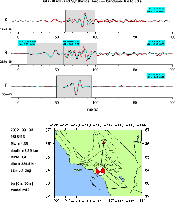
Test case seismograms with COMPUTE_ADJOINT_SOURCE = .false.. Plot shows a three-component seismogram: Z = vertical, R = radial, T = transverse. Black is the observed records, red is the synthetics, and blue is the reconstructed synthetics, made by applying the \(\Delta T\) and \(\Delta \ln A\) measurements within each window to the synthetics. No adjoint sources are plotted.
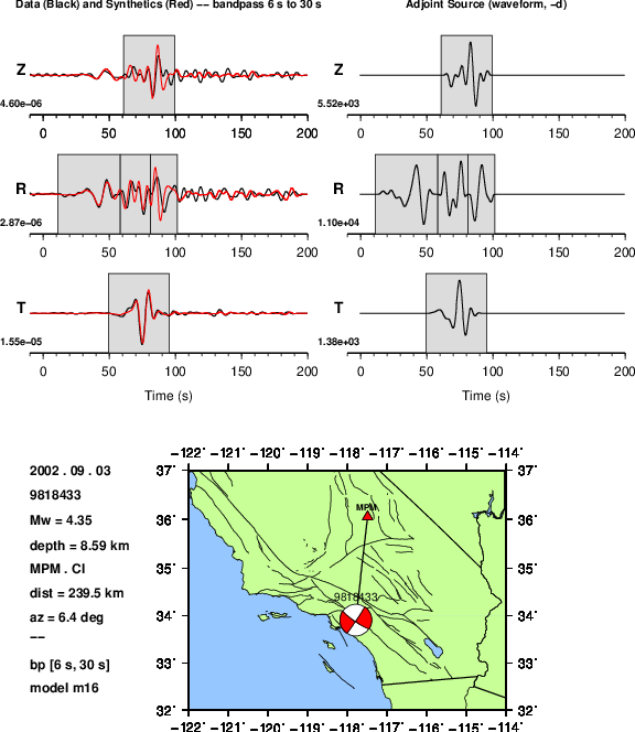
Left: Data (black), synthetics (red), and measurement windows.
Right: Adjoint sources constructed from the data alone imeas = 1, \(-d(t)/\|d(t)\|^2\)
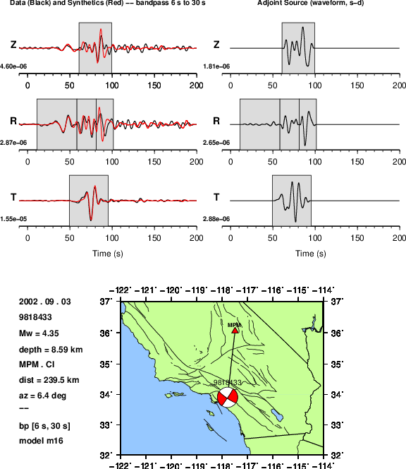
Left: Data (black), synthetics (red), and measurement windows.
Right: Adjoint sources for a waveform difference measurement imeas = 2, \(\mathbf{s} - \mathbf{d}\)
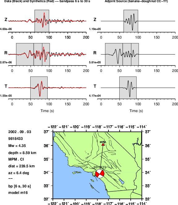
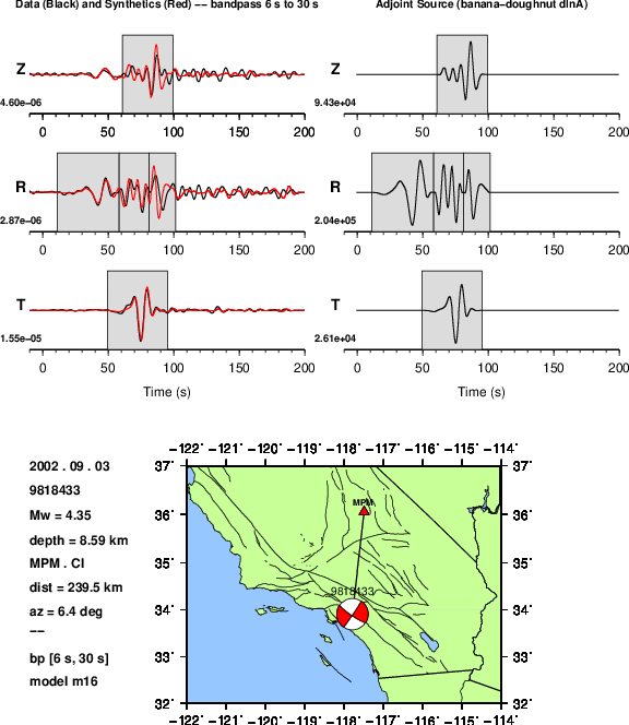
Left: Data (black), synthetics (red), and measurement windows.
Right: Adjoint sources for a sensitivity kernel based on a cross-correlation traveltime difference, \(\Delta T\) (imeas = 3).
Left: Data (black), synthetics (red), and measurement windows.
Right: Adjoint sources for a sensitivity kernel based on an amplitude difference, \(\Delta \ln A\) (imeas = 4).
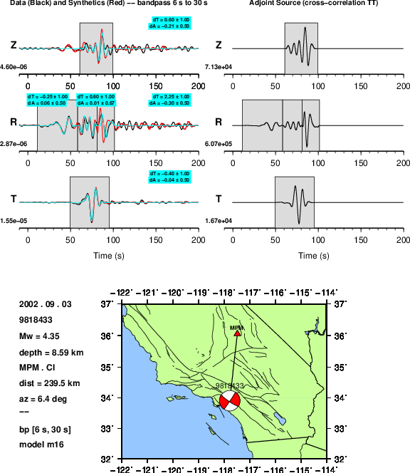
Left: Data (black), synthetics (red), and measurement windows.
Right: Adjoint sources for a cross-correlation traveltime difference, \(\Delta T\) (imeas = 5).

Left: Data (black), synthetics (red), and measurement windows.
Right: Adjoint sources for an amplitude difference, \(\Delta \ln A\) (imeas = 6).

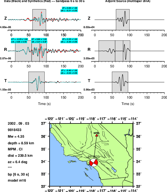
Left: Data (black), synthetics (red), and measurement windows.
Right: Adjoint sources for a multitaper traveltime difference (imeas = 7).
Left: Data (black), synthetics (red), and measurement windows.
Right: Adjoint sources for a multitaper amplitude difference (imeas = 8).
Reference
Vadim Monteiller, Stephen Beller, Bastien Plazolles, and Sébastien Chevrot. On the validity of the planar wave approximation to compute synthetic seismograms of teleseismic body waves in a 3-d regional model. Geophysical Journal International, 224(3):2060–2076, 2021.
J. Tromp, C. H. Tape, and Q. Liu. Seismic tomography, adjoint methods, time reversal and banana-doughnut kernels. Geophys. J. Int., 160:195–216, 2005. URL: http://scholar.google.com/scholar?hl=en\&btnG=Search\&q=intitle:Seismic+tomography,+adjoint+methods,+time+reversal+and+banana-doughnut+kernels\#0.
Q. Liu and J. Tromp. Finite-frequency kernels based on adjoint methods. Bull. Seism. Soc. Am., 96(6):2283–2397, 2006. URL: http://www.bssaonline.org/cgi/content/abstract/94/1/187.
C. H. Tape, Q. Liu, and J. Tromp. Finite-frequency tomography using adjoint methods - Methodology and examples using membrane surface waves. Geophys. J. Int., 168:1105–29, 2007.
C. H. Tape, Q. Liu, Alessia Maggi, and J. Tromp. Adjoint tomography of the southern California crust. Science, 325(5943):988–992, August 2009. URL: http://www.ncbi.nlm.nih.gov/pubmed/19696349, doi:10.1126/science.1175298.
A. Maggi, C. H. Tape, M. Chen, D. Chao, and J. Tromp. An automated time-window selection algorithm for seismic tomography. Geophys. J. Int., 178:257–281, July 2009. URL: http://blackwell-synergy.com/doi/abs/10.1111/j.1365-246X.2009.04099.x, doi:10.1111/j.1365-246X.2009.04099.x.
C. H. Tape. Seismic Tomography of Southern California Using Adjoint Methods. PhD thesis, Caltech, 2009. URL: http://thesis.library.caltech.edu/1656/.
C. H. Tape, Q. Liu, A. Maggi, and J. Tromp. Seismic tomography of the southern California crust based on spectral-element and adjoint methods. Geophys. J. Int., 180:433–462, 2010. URL: http://blackwell-synergy.com/doi/abs/10.1111/j.1365-246X.2009.04429.x, doi:10.1111/j.1365-246X.2009.04429.x.